Data processing of LEND collimated sensors
Author List:
W.V. Boynton1*, I.G. Mitrofanov2, D. Hamara1, D. Dean1, T.P. McClanahan3, A.B. Sanin2, M.L. Litvak2, G. Chin3, L.G. Evans4, K. Harshman1, J. Bodnarik1, A. Malakhov2, G. Milikh5, R. Sagdeev5, R. Starr6
Corresponding Author: wboynton@LPL.Arizona.edu
1Lunar and Planetary Laboratory, University of Arizona, Tucson, AZ, 85721 USA
2Institute for Space Research, RAS, Moscow 117997, RU
3Astrochemistry Laboratory, Code 691, NASA Goddard Space Flight Center, Greenbelt, MD, 20771, USA
4Computer Sciences Corporation, Lanham MD 20706, USA
5Space Physics Department, University of Maryland, College Park, MD, USA
6Catholic University, Washington
DC, USA
1. Introduction
This document serves to describe the process of generating Derived LEND Data (DLD) as archived in the PDS. It is taken from Boynton et al. (2012) with some corrections made to the equations provided in that work. That work inadvertently showed older versions of the equations that were not correct, though the data provided in that work did, in fact, use the data processing scheme as described below.
2. Reduction of LEND collimated sensor data
The LEND on board the Lunar Reconnaissance Orbiter (LRO) has continuously mapped the neutron flux from the Moon since July 2009. This section describes the step by step process used to reduce the raw collimated detector data into corrected DLD products.
2.1 Solar Energetic Particle events
Both the collimated and uncollimated sensors aboard LEND are sensitive to Solar Particle Events (SPEs). The onset of the SPE is obvious with a very rapid change in particle flux; the end of the event is defined as when the SPE count rate returns to the pre-event rate. We visually examine plots of raw data and residuals from corrected data (see sections 2.4 and 2.5), and monitor proton fluxes from GOES-13 [http://satdat.ngdc.noaa.gov/sem/goes/data/new_plots/2016/goes13/summary/] and ACE [http://www.srl.caltech.edu/ACE/ASC/DATA/level3/sis/Counts.cgi?LATEST=1] to identify SPEs and ignore LEND data associated with them. All count rates are assigned a value of -1 for records that occur in an SPE interval. A table of SPE intervals based on GOES-13 and ACE data over the duration of the mission is shown in table 1.
2.2 Outlier or off-limit events
The raw counts from the CSETN sensors are determined by adding the counts in channels 10 to 16. Occasionally, sporadic and randomly distributed ‘outlier’ values are seen in the raw detector count rates when summing channels 10 – 16. These outliers could be produced either due to some micro-discharge in the HV circuit of a counter, or due to some corruptions in the instrument memory. The data with outliers is excluded from the mapping data together with their associated time intervals. Histograms were constructed for each detector’s counts to ascertain a standard by which to call a particular record an ‘outlier’ event (figure 1). Based on these results, we set the limit on outlier values to be any detector record where the sum of the counts in channels 10 through 16 is greater than 11. Typically, a count rates of 12 cps or higher represents at least a seven-sigma event relative to the mean of about 1.25 cps. Detector records that are defined as outlier events are not used, and they are also assigned count rate values of -1 when converting to a derived record.
2.3 Off nadir measurements
Occasionally, particular instruments on board LRO have requested off nadir slews for targeted observations. The nadir angle--the angle between the LEND bore-sight and nadir vectors--is recorded for each raw record. If the nadir angle is greater than 1.9°, the record is ignored and a value of -1 is assigned to its count rate in the corresponding derived record.
2.4 Correction for instrument warm up
The LEND 3He sensors have a high sensitive volume and pressure of 20 atm. These sensors gradually increase in efficiency by 15 – 20 % after each of the approximately biweekly turn-on cycles due to accumulation of charge on the insulators that support the center electrode wire. Before this charge build-up, there is a dead volume at each end of the tube, but the charge build-up on the insulator essentially increases the active length of the center electrode and thus decreases the dead volume. A typical efficiency warm-up cycle for a collimated sensor is shown in figure 2.
Valid on-intervals are those intervals that are at least 5 days long. Data from the first six hours after turn on are not included in the processing to allow for occasional rapid change in detector efficiency. Records falling outside these valid intervals are not included in the orbital averaging or conversion to derived records. Outlier, off nadir, and SPE interval records are not used in the orbital averaging or in generating derived records.
Orbital average data are generated from all valid records taken pole-ward of 60° latitude to avoid variations due to maria at lower latitudes that show an enhancement due to fast neutrons. Curves are generated for each detector (i) for each ‘on’ interval (j) and are fit to an exponential,

where
t is the time since turn on, and Ai,j, ki,j,
and ![]() are fitting parameters (figure 2). The fits are
weighted by the reciprocal of the square of the standard error of the mean for
each orbital average. The constant Ai,j, is the counting rate
of the detector at efficiency saturation.
are fitting parameters (figure 2). The fits are
weighted by the reciprocal of the square of the standard error of the mean for
each orbital average. The constant Ai,j, is the counting rate
of the detector at efficiency saturation.
2.5 Correction for cosmic-ray variation
The solar cycle modulates the flux of galactic cosmic rays entering the solar system from elsewhere in the galaxy. As a consequence, the cosmic-ray flux in the inner solar system varies with time and is anti-correlated with the overall level of solar activity. Cosmic rays are the excitation source for lunar neutrons, so the LEND data must be normalized to their variation.
The ![]() values showed little variation over the first six ‘on’
periods (around 3 months), indicating that there was little change in the
cosmic-ray flux. These six values for each detector were averaged to generate
long-term normalization values,
values showed little variation over the first six ‘on’
periods (around 3 months), indicating that there was little change in the
cosmic-ray flux. These six values for each detector were averaged to generate
long-term normalization values, ![]() (table 2). Subsequent
(table 2). Subsequent ![]() values showed a gradual decrease over time due to the
lower cosmic-ray flux as solar activity increased; all subsequent data were
normalized by the ratio of the current
values showed a gradual decrease over time due to the
lower cosmic-ray flux as solar activity increased; all subsequent data were
normalized by the ratio of the current ![]() to its
to its ![]() . The adjusted count rate for each detector is given
by:
. The adjusted count rate for each detector is given
by:

where
![]() are the counts in detector i and the parenthetical
expression in the denominator adjusts for the change in detector efficiency due
to warm up. Because LEND counts over a 1-second accumulation time, the recorded
counts are simply converted directly to a rate; the count rates are so low that
no dead-time correction is needed.
are the counts in detector i and the parenthetical
expression in the denominator adjusts for the change in detector efficiency due
to warm up. Because LEND counts over a 1-second accumulation time, the recorded
counts are simply converted directly to a rate; the count rates are so low that
no dead-time correction is needed.
These ![]() values are also used as a measure of efficiency
differences between detectors when we have to adjust for a detector not
providing data for a given record, either because it is intentionally turned
off, or because it may have generated a count determined to be an outlier. For
these cases we take the average adjusted count rate for the “on” detectors and
assign that average rate to the “off” detectors with an adjustment for
differences in efficiency based on their
values are also used as a measure of efficiency
differences between detectors when we have to adjust for a detector not
providing data for a given record, either because it is intentionally turned
off, or because it may have generated a count determined to be an outlier. For
these cases we take the average adjusted count rate for the “on” detectors and
assign that average rate to the “off” detectors with an adjustment for
differences in efficiency based on their ![]() ratios. This adjustment is given as:
ratios. This adjustment is given as:

For example, if the adjusted count rates of detectors 1 and 2 are 1.25 cps and 2.20 cps, respectively, and detectors 3 and 4 are off, we find that the adjusted rate for detector 3 is (1.2426 * 3.45) / 2.3785 = 1.80 cps; similarly, the rate for detector 4 is 1.93 cps. The final adjusted count rate is simply the sum of the adjusted rate of all four detectors:

At this point, the data have been adjusted for changes in efficiency and for long-term changes in the cosmic-ray flux, but one additional correction needs to be made for short-term (10s of hours) changes in the cosmic-ray flux. Changes in the flux of cosmic rays can be seen both in the cosmic-ray flux at Earth and in occasional anomalies in the orbital average data relative to the fit of the warm-up efficiency function. Figure 2 shows an example of this effect seen in the residual to the warm-up efficiency fit. The residual is compared to the terrestrial cosmic-ray flux as measured at McMurdo, Antarctica [http://neutronm.bartol.udel.edu/], where a similar effect is seen. We take the residual to the warm up fits as a means to correct for short-term variations in the neutron flux. We are confident in this assignment because: (1) we see the same effects at the same time at both poles, (2) the effects are seen simultaneously in all four detectors, and (3) there is a significant correlation over the course of the mission between the McMurdo data and the residuals of the warm-up fits (significance > 99.9%).
Because we see the same effect over all four detectors, we make another fit to the orbital averages, but this time it is on the combined count-rate data from all four detectors to improve statistics. We generate smooth curves as a 24-hour moving average of the residuals, and this curve is then used for a point by point correction of each collimated record. Essentially the 24-hour-smoothed GCR variations get distributed back into each of the individual detector records. The short-term cosmic-ray correction factor (CRCF) is evaluated at each raw record’s collection time as
 (5)
(5)
For example, if the residual is 0.04 cps high and the value of the fit function is 4.00 cps, we multiply by
1 – (0.04/4) = 0.99 (6)
We find that the CRCF shows a standard deviation of about 1%, and thus it is an important correction to make because we are looking for count rate differences on the order of 0.01 cps or about 0.2%. The complete equation for the corrected count rate of each detector then becomes

2.6 Uncertainties on count rates
It is clear that the relative uncertainties on the corrected counts for any given record are significantly greater when one or more of the detectors is not producing valid data. In order to make maps, we need to calculate an average count rate of many records from a given location on the Moon. Thus we need to properly weight the data in calculating the average, e.g. a record in which four detectors return valid data must be given more weight than a record in which only two or three detectors return valid records.
We weight by the reciprocal of the variance, but estimating the variance with such a low number of counts is not straightforward. Normally one assumes the variance in the number of counts recorded is simply the number of counts. With a large number of counts, such an assumption is a reasonably good approximation to the true variance of the counts. It is important to remember, however, that the number of counts only yields our best estimate of the variance, s2, which is not generally equal to the true variance, σ2. For example, a record with 2 counts and one with 4 counts are both common occurrences, but the record with 2 counts would be given twice as much weight if the variance were simply taken as the number of counts. Such weighting gives a systematically low result.
This distinction is particularly important with LEND data since the counts in these records are so small. With the low counting rates present in our records, we must have a better means for estimating the variance. We use the value of the exponential efficiency function described above. This function is typically fit over a few hundred thousand records in each power ‘on’ cycle and is thus a much better estimate of the true variance at the time the data were collected. The variance on the number of counts is thus

Because we adjust the observed
count rates to account for instrument warm up and cosmic-ray variations, we
also have to adjust the observed variance. The variance, ![]() , for each valid detector record is thus
, for each valid detector record is thus

When one or more detectors fail to provide valid counts, their variance is calculated differently. The variance of an “off” detector is given by

If more than one detector is off, the sum of the counts due to all off detectors is

The sum of the counts due to all four detectors is

Note that the parenthetical expression is a constant. The variance on the total sum is thus

Continuing with the example at
equation 7, assuming the two ![]() for the on detectors are identical at 1.20 cps2.
The sum of all four adjusted count rates, R, is 7.18 cps, and
for the on detectors are identical at 1.20 cps2.
The sum of all four adjusted count rates, R, is 7.18 cps, and ![]() = 2.40 * (1+2.571/2.378)2, = 10.39 cps2,
showing that the uncertainty of the result is about double that of having all
four detectors returning valid data, in which case
= 2.40 * (1+2.571/2.378)2, = 10.39 cps2,
showing that the uncertainty of the result is about double that of having all
four detectors returning valid data, in which case ![]() = 4.8 cps2.
= 4.8 cps2.
In section 6 of Boynton et al. (2012) we independently calculate reduced chi squared values for 3263 different averages and show that our treatment of uncertainties is appropriate, i.e. the counting statistics as calculated here account for all observed random error in the observations.
References.
Boynton, W.V., G.F. Droege, I.G. Mitrofanov, T.P. McClanahan, A.B. Sanin, M.L. Litvak, M. Schaffner, G. Chin, L.G. Evans, J.B. Garvin, K. Harshman, A. Malakhov, G. Milikh, R. Sagdeev, and R. Starr (2012), High spatial resolution studies of epithermal neutron emission from the lunar poles: Constraints on hydrogen mobility, Journal of Geophysical Research - Planets 117, 1-19.
Tables
Table 1. UTC intervals in which data are excluded due to solar particle events (determined from GOES and ACE data)
|
SPE BEGIN |
SPE END |
||
|
9/15/2009 |
12:00:00 AM |
9/16/2009 |
12:00:00 AM |
|
9/27/2009 |
12:00:00 AM |
9/28/2009 |
12:00:00 AM |
|
10/11/2009 |
12:00:00 AM |
10/12/2009 |
12:00:00 AM |
|
10/21/2009 |
7:00:00 AM |
10/22/2009 |
7:00:00 PM |
|
10/23/2009 |
7:01:00 PM |
10/25/2009 |
12:00:00 AM |
|
11/6/2009 |
3:56:00 PM |
11/8/2009 |
12:00:00 AM |
|
11/14/2009 |
2:30:00 AM |
11/14/2009 |
7:15:00 PM |
|
11/20/2009 |
5:57:00 PM |
11/22/2009 |
12:00:00 AM |
|
11/25/2009 |
2:30:00 AM |
11/26/2009 |
5:00:00 AM |
|
11/30/2009 |
12:00:00 AM |
12/2/2009 |
12:00:00 AM |
|
12/5/2009 |
2:00:00 PM |
12/6/2009 |
6:00:00 PM |
|
1/13/2010 |
9:40:00 PM |
1/15/2010 |
3:50:00 PM |
|
1/20/2010 |
1:00:00 AM |
1/28/2010 |
12:32:00 PM |
|
2/7/2010 |
5:00:00 PM |
2/9/2010 |
7:00:00 AM |
|
4/5/2010 |
10:00:00 AM |
4/6/2010 |
3:00:00 PM |
|
6/12/2010 |
10:00:00 AM |
6/13/2010 |
12:00:00 AM |
|
8/3/2010 |
12:00:00 PM |
8/6/2010 |
3:00:00 PM |
|
8/6/2010 |
4:00:00 PM |
8/7/2010 |
12:00:00 AM |
|
8/14/2010 |
6:00:00 PM |
8/15/2010 |
12:00:00 PM |
|
8/18/2010 |
6:00:00 AM |
8/19/2010 |
12:00:00 PM |
|
1/28/2011 |
12:00:00 AM |
1/29/2011 |
12:00:00 AM |
|
2/14/2011 |
6:00:00 PM |
2/21/2011 |
12:00:00 AM |
|
3/7/2011 |
10:00:00 AM |
3/11/2011 |
12:00:00 PM |
|
3/21/2011 |
12:00:00 AM |
3/22/2011 |
12:00:00 AM |
|
3/21/2011 |
10:00:00 AM |
3/26/2011 |
10:00:00 AM |
|
4/4/2011 |
12:00:00 PM |
4/7/2011 |
12:00:00 PM |
|
5/11/2011 |
12:00:00 AM |
5/12/2011 |
12:00:00 AM |
|
5/21/2011 |
12:00:00 AM |
5/21/2011 |
12:00:00 PM |
|
6/4/2011 |
8:00:00 PM |
6/10/2011 |
12:00:00 AM |
|
8/2/2011 |
12:00:00 AM |
8/3/2011 |
12:00:00 AM |
|
8/4/2011 |
12:00:00 AM |
8/10/2011 |
6:00:00 PM |
|
9/6/2011 |
12:00:00 AM |
9/11/2011 |
12:00:00 AM |
|
9/17/2011 |
12:00:00 AM |
9/19/2011 |
12:00:00 PM |
|
9/22/2011 |
12:00:00 AM |
10/1/2011 |
12:00:00 AM |
|
10/3/2011 |
8:00:00 PM |
10/6/2011 |
12:00:00 AM |
|
10/22/2011 |
12:00:00 PM |
10/26/2011 |
12:00:00 AM |
|
11/3/2011 |
9:00:00 PM |
11/7/2011 |
12:00:00 AM |
|
11/26/2011 |
12:00:00 AM |
11/28/2011 |
12:00:00 AM |
|
12/25/2011 |
12:00:00 PM |
12/27/2011 |
12:00:00 AM |
|
1/22/2012 |
12:00:00 AM |
2/2/2012 |
12:00:00 AM |
|
3/7/2012 |
12:00:00 AM |
3/17/2012 |
12:00:00 AM |
|
5/17/2012 |
12:00:00 AM |
5/20/2012 |
12:00:00 AM |
|
5/26/2012 |
6:00:00 PM |
5/28/2012 |
12:00:00 AM |
|
6/16/2012 |
12:00:00 PM |
6/17/2012 |
12:00:00 PM |
|
7/6/2012 |
8:00:00 PM |
7/11/2012 |
12:00:00 PM |
|
7/17/2012 |
6:00:00 AM |
7/29/2012 |
12:00:00 AM |
|
9/1/2012 |
12:00:00 AM |
9/10/2012 |
12:00:00 AM |
|
9/26/2012 |
4:00:00 PM |
10/11/2012 |
3:00:00 PM |
|
11/8/2012 |
12:00:00 AM |
11/28/2012 |
12:00:00 AM |
|
3/5/2013 |
12:00:00 AM |
3/21/2013 |
3:00:00 PM |
|
4/11/2013 |
12:00:00 AM |
4/30/2013 |
12:00:00 AM |
|
5/13/2013 |
12:00:00 AM |
5/29/2013 |
12:00:00 AM |
|
6/12/2013 |
12:00:00 PM |
6/30/2013 |
12:00:00 AM |
|
8/20/2013 |
12:00:00 PM |
8/22/2013 |
12:00:00 PM |
|
9/30/2013 |
12:00:00 AM |
10/4/2013 |
12:00:00 AM |
|
10/28/2013 |
12:00:00 AM |
11/8/2013 |
12:00:00 AM |
|
11/19/2013 |
12:00:00 PM |
11/21/2013 |
12:00:00 AM |
|
12/15/2013 |
12:00:00 AM |
12/18/2013 |
12:00:00 AM |
|
12/26/2013 |
12:00:00 AM |
12/31/2013 |
12:00:00 AM |
|
1/6/2014 |
12:00:00 AM |
1/14/2014 |
12:00:00 AM |
|
2/20/2014 |
12:00:00 AM |
2/21/2014 |
12:00:00 AM |
|
2/25/2014 |
12:00:00 AM |
3/5/2014 |
12:00:00 AM |
|
3/29/2014 |
6:00:00 PM |
3/31/2014 |
12:00:00 AM |
|
4/18/2014 |
12:00:00 PM |
4/21/2014 |
12:00:00 AM |
|
8/25/2014 |
12:00:00 AM |
8/28/2014 |
12:00:00 AM |
|
9/1/2014 |
6:00:00 PM |
9/16/2014 |
12:00:00 AM |
|
9/22/2014 |
12:00:00 AM |
9/24/2014 |
12:00:00 AM |
|
9/25/2014 |
12:00:00 AM |
9/27/2014 |
12:00:00 AM |
|
11/1/2014 |
12:00:00 PM |
11/6/2014 |
12:00:00 AM |
|
12/13/2014 |
12:00:00 AM |
12/25/2014 |
12:00:00 AM |
|
2/21/2015 |
12:00:00 AM |
2/24/2015 |
12:00:00 AM |
|
3/15/2015 |
12:00:00 AM |
3/19/2015 |
12:00:00 AM |
|
3/24/2015 |
12:00:00 AM |
3/27/2015 |
12:00:00 AM |
|
4/22/2015 |
12:00:00 AM |
4/26/2015 |
12:00:00 AM |
|
5/11/2015 |
12:00:00 PM |
5/14/2015 |
12:00:00 AM |
|
5/27/2015 |
12:00:00 AM |
5/28/2015 |
12:00:00 AM |
|
6/18/2015 |
12:00:00 AM |
7/4/2015 |
12:00:00 AM |
|
9/20/2015 |
12:00:00 AM |
9/22/2015 |
12:00:00 AM |
|
10/7/2015 |
12:00:00 AM |
10/9/2015 |
12:00:00 AM |
|
10/29/2015 |
12:00:00 AM |
11/2/2015 |
12:00:00 AM |
|
11/9/2015 |
12:00:00 AM |
11/11/2015 |
12:00:00 PM |
Table 2. Average count rates of collimated detectors at the beginning of the mission (cps)
|
|
|
|
|
|
|
|


Figures.
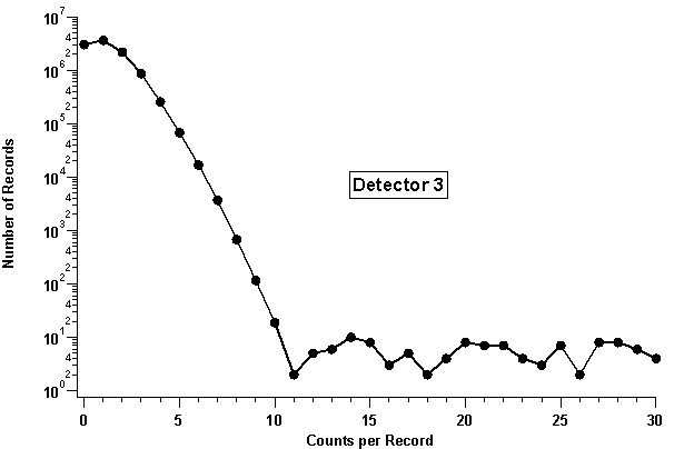
Figure 1. Histogram of total detector counts in channels 10 through 16. Records with counts > 11 are considered outlier values. They constitute only 0.01% of recorded events.
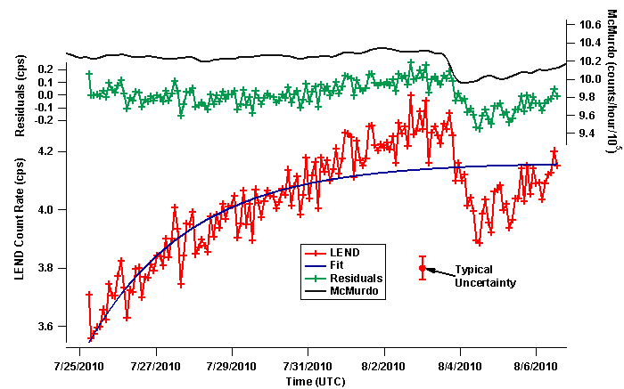
Figure 2. Typical warm up cycle based on the orbital average count rate of all collimated sensors. Fitting parameters are determined separately on each detector to correct for slightly different warm-up curves in each detector, but the orbital average of the sum of count rates in all four detectors (shown here) is used to correct for the short-term cosmic-ray variations. Deviations from the fit are due to short-term changes in the cosmic-ray flux as can be seen in these data from the McMurdo Antarctica cosmic-ray monitoring station. Corrections for short-term variations in the cosmic-ray flux are made based on a 24-hour moving average of the residuals. The McMurdo data are also 24-hour smoothed, and they have been interpolated to the same times as the LEND orbital averages. A typical error bar is shown for the standard error of the orbital averages. The scatter in the data is often larger than the error bar would suggest due to short-term cosmic-ray flux variations.