9 Smoothing of Engineering Data
GRS products produced prior to the 25 Feb. 2013 flight software upload use an engineering smoother process to detect and replace anomalous data points from the GRS engineering data. This process does not actually perform a traditional smoothing to remove noise. It is simply a tool for the detection and replacement of points that are statistical outliers. The engineering smoother process uses the “outliers” library from the R statistical package for outlier detection.
For each engineering channel four parameters are defined.
1. A search window size to look for outliers
2. A mean window size to generate replacement values
3. A statistical scoring method
4. A score threshold that separates the outliers
Table 2 shows the default values used for all engineering channels.
Table 2: Engineering smoother parameters
|
Name |
Value |
|
Search N |
50 |
|
Mean N |
50 |
|
Method |
Z |
|
Threshold |
5.0 |
Note that the actual search and mean windows include 2*N+1 points.
The algorithm proceeds by first calculating the "z" normal scores (differences between each value and the mean divided by the standard deviation) for every point in the search window. Then the results are checked to determine if the absolute value of the score at the window center exceeds the threshold. If so that point is replaced with the mean value of all points in the mean window who are not also outliers.
Data produced after the 25 Feb. 2013 flight software upload (SH3 and SCR) do not use the engineering smoother routine, in part because the time cadence of the data products changed notably following this upload and also because outlying data points were found not to be a notable issue.
10 Conversion of the MIDPOINT_MET to UTC_MIDPOINT_MET
The UTC conversion from the MIDPOINT_MET to UTC is handled by the SPICE toolkit using the following code:
partition = 1
sprintf(sclkch, “%d/%d”, partition, midpoint_met); // This creates a character string with
the partition number followed by ‘/’
followed by the midpoint_met
scs2e_c(sc_id, sclkch, j2000)
timout_c(j2000, 'YYYY MM DD HR:MN:SC.### ::UTC', 24, UTC_MIDPOINT_MET)
The routine scs2e_c converts the midpoint_met into ephemeris time j2000, whereby the spacecraft ID (sc_id), for MESSENGER is -236. The routine timout_c then converts the ephemeris time j2000 to a UTC time string which is associated with the observation.
For the SH3 and SCR data products, the ephemeris data are obtained from a call to READ_NS_SPICE(date, j2000_et), where the returned ephemeris data are sampled at times specified by the j2000_et parameter. This j2000_et parameter comes from the HK.MIDPOINT_J2000_ET field in the SHI data structure. HK.MIDPOINT_MET is also used as the MET field in the final new SHIELD data structure.
11 Spatial Data Calculation
For the HPGE_RAW, HPGE_AC and HPGE_SH data products the following spatial data is calculated:
DELTA_ANGLE
INSTRBORESIGHT_MERCURY
INTERSECTION
LOCAL_HOUR
LOCAL_MINUTE
MERCURY_CENTRIC_LATITUDE
MERCURY_CENTRIC_LONGITUDE
MERCURY_SOL
POINTING
SCALT
The SH3 and SCR products also include the following spatial data:
VEL_VECTOR
VEL_NORM
BETA_ANGLE
SUN_DISTANCE
These calculations are performed for the j2000 value of the MIDPOINT_MET. The conversion from the midpoint_met to j2000 is handled by the SPICE toolkit using the following code:
partition = 1
sprintf(sclkch, “%d/%d”, partition, midpoint_met); // This creates a character string with
the partition number followed by ‘/’
followed by the midpoint_met
scs2e_c(sc_id, sclkch, j2000)
The routine scs2e_c converts the midpoint_met into ephemeris time j2000, whereby the spacecraft ID (sc_id) for MESSENGER is -236.
11.1 SCALT Calculation
Find the sub-spacecraft point of MESSENGER on the surface of Mercury using the “Intercept” method (point on the surface of Mercury on a line between MESSENGER and the center of Mercury) and find the spacecraft altitude, SCALT. This is handled by the SPICE toolkit using the following code:
subpt_c(“Intercept”, “Mercury”, j2000, “NONE”, “MESSENGER”,
spoint, SCALT)
The returned value spoint is an array with the sub-spacecraft point on the surface of Mercury at time of j2000 and the returned value SC_ALT is a reference to the altitude of MESSENGER at the time of j2000.
11.2 MERCURY_CENTRIC_LATITUDE and MERCURY_CENTRIC_LONGITUDE Calculation
Convert the sub-spacecraft point of MESSENGER on the surface of Mercury into latitude and longitude along with the radii of Mercury. This is handled by the SPICE toolkit using the following code:
reclat_c(spoint, mercury_radii, MERCURY_CENTRIC_LONGITUDE,
MERCURY_CENTRIC_LATITUDE)
where spoint is the array with the point on the surface of Mercury returned in the subpt_c call from the SCALT calculation above.
The returned value mercury_radii is an array with the radii of Mercury, the returned value MERCURY_CENTRIC_LONGITUDE is a reference to the longitude of Mercury at the point on the surface of Mercury under MESSENGER and the returned value MERCURY_CENTRIC_LATITUDE is a reference to the latitude at the point on the surface of Mercury under MESSENGER.
The longitude and latitude are converted to degrees from radians by multiplying them by 180.0 and dividing that product by PI.
11.3 POINTING Calculation
Check if a SPICE CK kernel file, the SPICE kernel with spacecraft orientation information, contains data for the j2000 value.
For performing this, convert the j2000 value to spacecraft clock (‘ticks’). The conversion from the j2000 to ticks is handled by the SPICE toolkit using the following code:
sce2t_c(sc_id, j2000, ticks)
The routine sce2t_c converts the j2000 value into spacecraft clock (‘ticks’), whereby the spacecraft ID for MESSENGER is -236.
The orientation of MESSENGER is obtained by calling the SPICE ck kernel using the current spacecraft clock to get pointing info with the api as follows:
ckgp_c(sc_ck_id, ticks, 0.0, “J2000”, matrix, clckout, found)
where sc_ck_id is the spacecraft CK SPICE kernel id of -236000.
If the orientation data exists for the spacecraft clock then the following step occur:
POINTING is set to 1.
If the orientation data does not exist for the spacecraft clock then the following step occur:
POINTING is set to 0.
11.4 INSTRBORESIGHT_MERCURY, INTERSECTION Calculation
If the SPICE orientation data exists at time j2000 as determined in the previous step then perform the following steps:
1. Get the position of MESSENGER as seen from Mercury in the inertial frame, J2000. This is handled by the SPICE toolkit using the following code:
spkezr_c(“MESSENGER”, j2000, “J2000”, “NONE”, “MERCURY”,
state, lt)
vequ_c(state[0], scpos_body)
2. Get the transformation matrix from the instrument frame, “MSGR_GRNS_GRS”, to the body-fixed rotating frame, “J2000”, at time j2000 using the following code:
pxform_c(“MSGR_GRNS_GRS”, “IAU_MERCURY”, j2000, instr2body)
3. Find the instrument “boresight” direction to the body-fixed frame using the following code:
vpack(0.0, 0.0, 1.0, bsight_instr)
mxv_c(instr2body, bsight_instr, bsight_body)
4. Find the INSTRBORESIGHT_MERCURY with the following code:
surfpt_c(scpos_body, bsight_body, mercury_radii[0], mercury_radii[1],
mercury_radii[2], INSTRBORESIGHT_MERCURY, found)
where scpos_body is first three elements in the state array returned in the call to spkezr_c
from a an earlier step.
5. If the INSTRBORESIGHT_MERCURY is found then INTERSECTION is set to 1 else INTERSECTION is set to 0.
6. If the SPICE orientation data for time j2000 does not exist then INSTRBORESIGHT_MERCURY is set to an array of 0.0, 0.0, 0.0 and INTERSECTING is set to 0.
11.5 DELTA_ANGLE Calculation
Find the DELTA_ANGLE using the following steps:
If the INSTRBORESIGHT_MERCURY is found then
1. Find the radii of Mercury:
bodvar_c(199, “RADII”, n, radii)
where 199 is the body id of Mercury.
2. Find the normal to Mercury at the surface:
surfnm_c(radii[0], radii[1], radii[2], INSTRBORESIGHT_MERCURY, normal)
3. Create a vector representing north using the following code:
vpack(0.0, 0.0, 1.0, north)
4. Find the transformation matrix, body2local, having the normal to the surface of Mercury as a +Z axis and having the north vector lying on the X plane with the following code:
twovec_c(normal, 3, north, 1, body2local)
5. Create vector representing instrument reference direction, +Y axis of instrument head frame:
vpack(0.0, 1.0, 0.0, refdir_instr)
6. Rotate the instrument reference direction to the local level frame using the following code:
mxv_c(instr2body, refdir_instr, refdir_body)
mxv_c(body2local, refdir_body, refdir_local)
where instr2body and body2local are the transformation matrices returned in previous steps.
7. Convert rectangle coordinates to range, right ascension, DELTA_ANGLE, and declination:
recrad_c(refdir_local, range, DELTA_ANGLE, dec)
where range is a reference to the range, DELTA_ANGLE is a reference to the right ascension
and dec is a reference to the declination.
The DELTA_ANGLE is converted to degrees from radians by multiplying it by 180.0 and
dividing that product by PI.
If the INSTRBORESIGHT_MERCURY is not found then
1. Set DELTA_ANGLE to 0.0.
11.6 LOCAL_HOUR, LOCAL_MIN Calculation
If the orientation information was found in a previous step then
Get local hour, LOCAL_HOUR, and the local minute, LOCAL_MIN, at the longitude of the
sub-point of MESSENGER on the surface of Mercury with the following code:
et2lst(j2000, 199, MERCURY_LONGITUDE, “Planetocentric”,
LOCAL_HOUR, LOCAL_MIN, local_second,
localtime, local_ampm,14, 40, 5)
where 199 is the body id of Mercury and MERCURY_LONGITUDE is from an above step.
If the orientation information was not found in a previous step then LOCAL_HOUR and LOCAL_MIN are set to 0.
11.7 MERCURY_SOL Calculation
Get the MERCURY_SOL, the longitude of the Sun, as seen from Mercury at the time j2000, in degrees using the following code:
MERCURY_SOL = dpr_c() * lspcn_c(“MERCURY”, j2000, “NONE”)
where dpr_c is a SPICE call that returns the number of degrees per radian and lspcn_c is the
SPICE call that computes the longitude of the Sun as seen from a specified body.
11.8 VEL_VECTOR_J2000 and VEL_NORM Calculations
The appropriate SPICE CD kernel file is read using the cspice_furnsh subroutine. The vector velocity of the MESSENGER spacecraft with respect to Mercury (or Venus for Venus flyby data) in the J2000 reference frame is a temporary data value, and is found using:
cspice_spkezr,'MESSENGER',j2000_et,'J2000','LT+S',’Mercury’,posvel,ltime
where posvel is a 6-element, time-dependent vector. The last three elements contain the three vector velocity components in the J2000 reference frame:
vel_vector_j2000 = posvel[3:*,*]
A description of how this J2000 velocity vector is transformed into the nadir-fixed coordinate system is described below in Section 8.5. The scalar velocity vel_norm is calculated as a loop over the number of elements in j2000_et:
vel_norm = fltarr(n_elements(j2000_et))
for i=0,n_elements(j2000_et)-1 do $
vel_norm[i] = cspice_vnorm(vel[*,i])
11.9 VEL_VECTOR Calculation
To calculate the vector velocity in the nadir-fixed coordinate system, the following steps need to be completed: 1) calculate a rotation matrix from Mercury into the J2000 reference frame, so that the spacecraft (x,y,z) position vector (spoint), which was returned in the Mercury reference frame, can be transformed into the J2000 reference frame. 2) Calculate unit vectors in the nadir-fixed reference frame. 3) Transform the vector velocity into the nadir-fixed reference frame by calculating a 9-element transformation matrix using direction cosines between the unit vectors in different coordinate systems. 4) Transform the vector velocity from J2000 reference frame into the nadir-fixed reference using this 9-element transformation matrix.
The Mercury to J2000 rotation matrix is obtained using:
cspice_pxform,'IAU_MERCURY','J2000',j2000_et,pform_mer_j2000
where pform_mer_j2000 is the transformation matrix. The planet-to-spacecraft vector in the Mercury reference frame is spoint (which was calculated in Section 8.2), and is transformed to the J2000 frame using:
r_j2000 = fltarr(3,n_elements(j2000_et))
for i=0,n_elements(fsp)-1 do begin
cspice_mxv,pform_mer_j2000[*,*,i],spoint[*,i],tmp
r_j2000[*,i] = tmp
endfor
Now the nadir-fixed coordinate system is defined as given in Section 3, where the z-axis is the spacecraft-to-Mercury vector (i.e., the negative of the Mercury-to-spacecraft vector). The other axes are obtained via cross products:
nadir_z = -r_j2000
nadir_x = fltarr(3,n_elements(j2000_et))
nadir_y = fltarr(3,n_elements(j2000_et))
for i=0,n_elements(j2000_et)-1 do begin
; normalize the z-axis
nadir_z[*,i] = nadir_z[*,i]/cspice_vnorm(nadir_z[*,i])
; the y-axis is the cross product of the z with the velocity
nadir_y[*,i] = crossp(nadir_z[*,i],vel[*,i])
nadir_y[*,i] = nadir_y[*,i]/cspice_vnorm(nadir_y[*,i])
; the x-axis is the cross product with the y axis
nadir_x[*,i] = crossp(nadir_y[*,i],nadir_z[*,i])
nadir_x[*,i] = nadir_x[*,i]/cspice_vnorm(nadir_x[*,i])
endfor
Finally, a 9-element transformation matrix of direction cosines is calculated in the same loop as the final vec_velocity value in the nadir-fixed coordinate system (NOTE: since the direction cosines are calculated using a cosine calculation between two vectors, the spacecraft fixed unit vectors, xaxis_sc, work just as well as the J2000 x-axis vectors xaxis_j2000):
vel_vector = fltarr(3,n_elements(j2000_et))
trans2 = fltarr(3,3,n_elements(j2000_et))
for i=0,n_elements(j2000_et)-1 do begin
xxd = cos(cspice_vsep(xaxis_sc,nadir_x[*,i]))
xyd = cos(cspice_vsep(xaxis_sc,nadir_y[*,i]))
xzd = cos(cspice_vsep(xaxis_sc,nadir_z[*,i]))
yxd = cos(cspice_vsep(yaxis_sc,nadir_x[*,i]))
yyd = cos(cspice_vsep(yaxis_sc,nadir_y[*,i]))
yzd = cos(cspice_vsep(yaxis_sc,nadir_z[*,i]))
zxd = cos(cspice_vsep(zaxis_sc,nadir_x[*,i]))
zyd = cos(cspice_vsep(zaxis_sc,nadir_y[*,i]))
zzd = cos(cspice_vsep(zaxis_sc,nadir_z[*,i]))
trans_tmp = [[xxd,xyd,xzd],[yxd,yyd,yzd],[zxd,zyd,zzd]]
trans2[*,*,i] = trans_tmp
vel_vector[*,i] = trans_tmp#vel[*,i]
endfor
12 Spacecraft Orientation Calculation
For the HPGE_RAW, HPGE_AC and HPGE_SH data products the following spacecraft orientation data is calculated:
NADIR_ANGLE
AZIMUTH
TWIST_ANGLE
POINTING_FLAG
For the SH3 and SCR data products, the following spacecraft orientation data is also calculated:
V_DOT_X
V_DOT_Y
V_DOT_Z
SC_TO_NADIR_ROT
These calculations are performed for the j2000 value of the MIDPOINT_MET within the MSGR_LVLH frame which has a value of -236910 and the MSGR_SPACECRAFT frame which has a value of -236000 using the following steps:
1. Initialize the pointing_flag, nadir_angle, azimuth and twist_angles:
POINTING_FLAG = 0
NADIR_ANGLE = 0.0
AZIMUTH = 0.0
TWIST_ANGLE = 0.0
2. Check for CK kernel file having data for the j2000 value of the MIDPOINT_MET:
sce2t_c(SCID, et, &dpsclk)
ckgp_c(sc_ck_id, dpsclk, 0.0, “J2000”, matrix, clckout, found)
where SCID is the spacecraft id of -236, sc_ck_id is the spacecraft CK SPICE kernel id of
-236000.
If found is 1 then the following steps occur:
POINTING_FLAG is set to 1.
Go to the next step.
If found is not 1 then the following steps occur:
POINTING_FLAG is set to 0.
Stop processing.
3. Get the transformation matrix from the MSGR_LVLH frame to the MSGR_SPACECRAFT
frame at time j2000 using the following code:
pxform_c(“MSGR_LVLH”, “MSGR_SPACECRAFT”, j2000, sc_dynamic_frame2sc_frame)
4. Get the twist angle, elevation angle and azimuth at time j2000 using the following code:
m2eul_c(sc_dynamic_frame2sc_frame, 3, 1, 3, TWIST_ANGLE, elevation_angle, AZIMUTH)
where the sc_dynamic_frame2sc_frame was derived in the previous step.
5. Make sure that the azimuth, elevation angle and twist angle are within valid ranges (azimuth is between 0, 2 *PI, elevation angle is between, -PI/2, PI/2 and twist angle is between 0, 2 * PI) using the following code:
AZIMUTH = AZIMUTH – PI/2
elevation_angle = PI/2 – elevation_angle
if (AZIMUTH < 0.0)
{
AZIMUTH = AZIMUTH + 2 *PI
}
if (TWIST_ANGLE < 0.0)
{
TWIST_ANGLE = TWIST_ANGLE + 2 *PI
}
6. Derive the nadir angle from the elevation angle using the following code:
NADIR_ANGLE = elevation_angle + PI/2
7. Convert the nadir angle, azimuth and twist angles from radians to degrees using the following code:
NADIR_ANGLE = NADIR_ANGLE * DEGS_IN_RAD
AZIMUTH = AZIMUTH * DEGS_IN_RAD
TWIST_ANGLE = TWIST_ANGLE * DEGS_IN_RAD
where DEGS_IN_RAD is 57.295779513.
12.1 V_DOT_X Calculation
v_dot_x is the dot product of the spacecraft vector velocity with the spacecraft x-axis direction in the spacecraft fixed reference frame. For the purposes of the NS calculation, the spacecraft x-axis is the normal to NS LG1 sensor, as described in Section 3. To obtain this dot product, the spacecraft unit vector directions and the spacecraft vector velocity need to be in the same reference frame, the J2000 frame. First, unit vectors for the spacecraft fixed frame are defined:
xaxis_sc = double([1,0,0])
yaxis_sc = double([0,1,0])
zaxis_sc = double([0,0,1])
Next, a rotation matrix from the MESSENGER fixed reference frame to the J2000 reference frame is calculated:
cspice_pxform,'MSGR_SPACECRAFT','J2000',j2000_et,pform
where pform is the time-dependent transformation matrix. A new set of x, y, and z vectors are defined:
xaxis_j2000 = fltarr(3,n_elements(j2000_et))
yaxis_j2000 = fltarr(3,n_elements(j2000_et))
zaxis_j2000 = fltarr(3,n_elements(j2000_et))
and within a loop, the rotation matrix is applied to spacecraft unit vectors:
for i=0,n_elements(j2000_et)-1 do begin
cspice_mxv,pform[*,*,i],xaxis_sc,tmp
xaxis_j2000[*,i] = tmp
cspice_mxv,pform[*,*,i],yaxis_sc,tmp
yaxis_j2000[*,i] = tmp
cspice_mxv,pform[*,*,i],zaxis_sc,tmp
zaxis_j2000[*,i] = tmp
endfor
Now, both the vector velocity and spacecraft unit vectors are in the J2000 reference frame. The normalized dot product of the vector velocity with the spacecraft x-axis can now be calculated:
v_dot_x = fltarr(n_elements(j2000_et))
for i=0,n_elements(j2000_et)-1 do $
v_dot_x[i] = cspice_vdot(xaxis_j2000[*,i],vel[*,i])/cspice_vnorm[*,i])
This process is releated for v_dot_y and v_dot_z by looping over 0 to n_elements(j2000_et) – 1 for
v_dot_y[i] = cspice_vdot(yaxis_j2000[*,i],vel[*,i])/cspice_vnorm[*,i])
and
v_dot_z[i] = cspice_vdot(zaxis_j2000[*,i],vel[*,i])/cspice_vnorm[*,i])
respectively.
12.2 SC_TO_NADIR_ROT Calculation
A 9-element transformation matrix between the spacecraft fixed coordinate system and the nadir fixed coordinate system is calculated with direction cosines:
sc_to_nadir_rot = fltarr(3,3,n_elements(j2000_et))
for i=0,n_elements(j2000_et)-1 do begin
xxd = cos(cspice_vsep(nadir_x[*,i],xaxis_j2000[*,i]))
yxd = cos(cspice_vsep(nadir_y[*,i],xaxis_j2000[*,i]))
zxd = cos(cspice_vsep(nadir_z[*,i],xaxis_j2000[*,i]))
xyd = cos(cspice_vsep(nadir_x[*,i],yaxis_j2000[*,i]))
yyd = cos(cspice_vsep(nadir_y[*,i],yaxis_j2000[*,i]))
zyd = cos(cspice_vsep(nadir_z[*,i],yaxis_j2000[*,i]))
xzd = cos(cspice_vsep(nadir_x[*,i],zaxis_j2000[*,i]))
yzd = cos(cspice_vsep(nadir_y[*,i],zaxis_j2000[*,i]))
zzd = cos(cspice_vsep(nadir_z[*,i],zaxis_j2000[*,i]))
trans_tmp = [[xxd,xyd,xzd],[yxd,yyd,yzd],[zxd,zyd,zzd]]
trans[*,*,i] = trans_tmp
endfor
13 Engineering Data Interpolation at MIDPOINT_MET for GRS_CAL_RAW, GRS_CAL_AC and GRS_CAL_SH
For the CDR data products GRS_CAL_RAW, GRS_CAL_AC and GRS_CAL_SH engineering data at the time of the measurement is recorded. To get the associated engineering readings, data is returned from the GRS_ENG_TAB database table for the MIDPOINT_MET of the measurement by either returning the engineering data at the MIDPOINT_MET if it exists or by returning the interpolation of the engineering data at the MIDPOINT MET. This is described by the following:
1. Get the values of the first record in GRS_ENG_TAB with a MET <= MIDPOINT_MET
where the records are ordered in descending MET order. This is the record with the time
closest to the MIDPOINT_MET with the MET earlier or equal to the MIDPOINT_MET.
2. If the record with the MET closest to the MIDPOINT_MET with a MET <=
MIDPOINT_MET is not found then try to get the values of the first record in the
GRS_ENG_TAB with a MET > MIDPOINT_MET where the records are ordered in
ascending order. This is the record with the MET closest to the MIDPOINT_MET with the
MET later than the MIDPOINT_MET. If a record is found then the smoothed engineering
values from this record are used.
3. If the record with the MET closest to the MIDPOINT_MET with the MET earlier or equal to
the MIDPOINT_MET is found then if the MET of this record is the MIDPOINT_MET then
smoothed engineering values from this record are used.
4. If the record with the MET closest to the MIDPOINT_MET with the MET <=
MIDPOINT_MET is found and the MET of this record is not the MIDPOINT_MET
then try to get the values of the first record in the GRS_ENG_TAB with a MET >
MIDPOINT_MET where the records are ordered in ascending order. This is the record with
the MET closest to the MIDPOINT_MET with the MET later than the MIDPOINT_MET. If
no record is found then the smoothed engineering values from the record with the MET
closest to the MIDPOINT_MET with the MET < MIDPOINT_MET are used.
5. If a record exists with the MET closest to the MIDPOINT_MET with a MET <
MIDPOINT_MET and a record exists with the closest MET with the MET >
MIDPOINT_MET then the smoothed engineering data is interpolated using the following
formula:
interpolated_smoothed_value = smoothed_value_1 + (((MIDPOINT_MET - MET_1) *
(smoothed_value_2-smoothed_value_1))/
(MET_2 - MET_1))
where the parameters with “_1” correspond to the GRS_ENG_TAB record with a MET <
MIDPOINT_MET and the parameters with “_2” correspond to the GRS_ENG_TAB record
with a MET > MIDPOINT_MET.
For the HPGE_RAW and HPGE_AC data products, the GRS_ENG_TAB columns returned are the smoothed data for:
HPGE_TEMP_1
HPGE_TEMP_2
CALIB_AVG_DET_TEMP
PREAMP_TEMP
SHAPER_TEMP
HV_MONITOR
For SHIELD data product, the GRS_ENG_TAB columns returned are the smoothed data for:
AD_TEMP
HVPS_TEMP
HVPS_VOLT
HVPS_REF_VOLT
PREAMP_TEMP
SHAPER_TEMP
HV_MONITOR
For the shield data products produced after the 25 Feb. 2013 flight software upload (SH3 and SCR), smoothed engineering data from the GRS STA file for:
PREAMP_TEMP,
SHAPER_TEMP
are included. The STA data were sampled on a slower time cadence than the other data structures, so a linear interpolation of these four fields onto the SLR JDAY cadence was performed. The interpolated values for the MET_MIDPOINT times for each CDR were used for the CDR values in these fields.
14 Software Counters Closest to MIDPOINT_MET for GRS_CAL_RAW, GRS_CAL_AC and GRS_CAL_SH
For the GRS_CAL_RAW , GRS_CAL_AC and GRS_CAL_SH data products software counter data from the GRS_SWC_TAB database table is returned for the MIDPOINT_MET by returning the software counter data at the MIDPOINT_MET if it exists else by returning the software counter data closest in time to the MIDPOINT MET. This is described by the following:
1. Get the values of the first record in GRS_SWC_TAB with a MET <= MIDPOINT_MET
where the records are ordered in descending MET order. This is the record with the MET
closest to the MIDPOINT_MET with the MET earlier or equal to the MIDPOINT_MET.
2. If the record with the MET closest to the MIDPOINT_MET with the MET <=
MIDPOINT_MET is not found then try to get the values of the first record in the
GRS_ENG_TAB with a MET > MIDPOINT_MET where the records are ordered in
ascending order. This is the record with the MET closest to the MIDPOINT_MET with the
MET later than the MIDPOINT_MET. If a record is found then the software counter values
from this record are used.
3. If the record with the MET closest to the MIDPOINT_MET with the MET earlier or equal to
the MIDPOINT_MET is found then if the MET of this record is the MIDPOINT_MET then
software counters values from this record are used.
4. If the record with the MET closest to the MIDPOINT_MET with the MET <= MIDPOINT_MET is found then if the MET of this record is not the MIDPOINT_MET then try to get the values of the first record in the GRS_SWC_TAB with a MET > MIDPOINT_MET where the records are ordered in ascending order. This is the record with the MET closest to the MIDPOINT_MET with the MET later than the MIDPOINT_MET. If no record is found then the software counter values from the record with the MET closest to the MIDPOINT_MET with the MET < MIDPOINT_MET are used.
5. If a record exists with the MET closest to the MIDPOINT_MET with a MET earlier than the MIDPOINT_MET and a record exists with the closest MET with the MET > MIDPOINT_MET then the software counter data values from the record with a MET closest to the MIDPOINT_MET are used.
For the GRS_CAL_RAW and GRS_CAL_AC data products, the GRS_SWC_TAB columns returned are for the software counter data for:
HPGE_RAW_EVENTS
SHIELD_RAW_EVENTS
ACCUMULATED_DEAD_TIME
HPGE_CHARGE_RESETS
SHEILD_CHARGE_RESETS
ALL_EVENTS
ALL_CH0_CH1_EVENTS
ALL_CH0_EVENTS
ALL_CH1_EVENTS
INVALID_SINGLE_CH0
INVALID_SINGLE_CH1
INVALID_COINCIDENT_CH0
INVALID_COINCIDENT_CH1
VALID_SINGLE_CH0
VALID_COINCIDENT_CH0
VALID_SINGLE_CH1
VALID_COINCIDENT_CH1
ALL_VALID_COINCIDENT
INVERTED_CH0
CH0_PILEUP_REJECT
FIFO_FULL_COUNT
PULSER_ENERGY_SUM
PULSER_ENERGY _SUM2
PULSER_EVENTS
INVALID_PULSER_EVENTS
NEUTRON_EVENTS
PULSER_OFFSET.
For GRS_CAL_SH data product, the GRS_SWC_TAB columns returned are for the software counter data for:
HPGE_RAW_EVENTS_1
SHIELD_RAW_EVENTS_1
ACCUMULATED_DEAD_TIME_1
For the shield data products produced after the 25 Feb. 2013 flight software upload (SH3 and SCR), smoothed scalar count rate data from the GRS STA file for:
SHLD_CHRG_RSET_1SEC
ACCUMULATED_DEAD_TIME
are included. ACCUMULATED_DEAD_TIME itself is not reported in the CDRs, but is used to derive the DEADTIME_FRAC value that is reported. Section 8 details the derivation of DEADTIME_FRAC from ACCUMULATED_DEAD_TIME. Also included in the CDRs are the:
TRIPLE_TMP
scaler value from the neutron spectrometer FSP (Full Science Packet) data product.
The STA and FSP data were sampled on a slower time cadence than the other data structures, so a linear interpolation of these four fields onto the SLR JDAY cadence was performed. The interpolated values for the MET_MIDPOINT times for each CDR were used for the CDR values in these fields.
15 Spectral Correction
Spectral corrections are performed for the GRS_RAW and GRS_ANC products. The MESSENGER Gamma Ray Spectrometer exhibits gain drifts with temperature. These drifts are due to different subsystems located in different parts of the instrument. The three major components whose temperatures contribute to these errors are the detector, the preamp, and the shaper amp. The contributions of each of these components were individually characterized prior to launch and are documented in the cal report. For each subsystem, a polynomial was generated that gives the percent change in the gain of that subsystem as a function of that subsystem’s temperature.
In order to effectively add together individual collection intervals, they must all have a common gain and offset to prevent line broadening due to misalignment of the peaks in the different spectra. Since there are not enough counts in any given spectrum to establish a calibration, we must calculate the gain and offset based on the measured temperatures of the various subsystems, then re-bin the counts in each spectrum to align the channels in all of the spectra prior to summing them.
Each channel in the spectrum does not represent a single, unique energy, but rather a range of energies such that any gamma ray where channel_low_limit £ gamma_energy < channel_high_limit is counted in this channel. We use the temperatures of the subsystems and the polynomials to calculate the low and high energies for each of the input channels, then we use a desired output gain and offset to calculate the low and high energies for the output channels, then we map the counts from input to output based on those limits.
The input channel ranges are calculated from the polynomials as follows (see sections 15.1 and 15.2 for the values for the parameters and coefficients):
actual_gain = gain_at_norm_temp / (poly(preamp_coef, preamp_temp) * poly(shaper_coef, shaper_temp))
Input_limit[k] = (k – 0.5) * actual_gain
and for the output channel ranges:
output_limit[k] = (k – 0.5) * desired_gain
Since the detector temperature is very tightly controlled, we do not currently do any correction for detector temperature. Additionally, no offset drifts were identified during calibration that would need to be corrected.
Figure 1 and Figure 2 illustrate the process of mapping the counts from the instrument channel space to a new channel space.
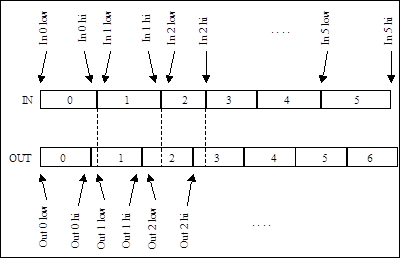
Figure 1: Input channels larger than output channels
As you can see in Figure 1, the counts the instrument puts in channel 0 should really be divided between channel 0 and channel 1. Knowing the high (hi) and low limits of the input and output channel we can divide up the counts as follows:
![]()
![]()
![]()
Then for input channel 1 the process is
![]()
![]()
![]()
In Figure 1 the output bins are generally smaller than the input bins. Figure 2 illustrates the case where the output channels are generally wider than the input channels.

Figure 2: Input channels smaller than output channels
In this case the process becomes
![]()
![]()
![]()
And for channel 1
![]()
![]()
![]()
![]()
![]()
As you can see, the process is different for different alignments of the input and output channels. These can be generalized into 2 cases distinguished by the relative positions of the high limits of the input and output channels. These 2 cases are illustrated in Figure 3 and Figure 4. Since we attempted to set the instrument gain very close to the desired gain, we will have likely oscillated between these 2 cases as the temperatures of the various subsystems change.

Figure 3: Algorithm for the case out_hi £ in_hi

Figure 4: Algorithm for the case out_hi > in_hi
15.1 preamp_coef
The preamp correction polynomial coefficients were determined during pre-launch characterization.
|
C4 |
-4.5335E-11 |
|
C3 |
-2.0620E-10 |
|
C2 |
6.1457E-07 |
|
C1 |
4.8884E-05 |
|
C0 |
1.0000E+00 |
15.2 shaper_coef
The shaper amp correction polynomial coefficients were determined during pre-launch characterization.
|
C4 |
9.8926E-12 |
|
C3 |
7.7979E-10 |
|
C2 |
-2.5824E-07 |
|
C1 |
-1.2509E-05 |
|
C0 |
1.0004E+00 |
15.3 gain_at_norm_temp
Since the polynomials give the percentage change in gain with temperature, we need a reference point from which to calculate the current gain. This reference point is the gain of the system when the temperatures are such that all of the polynomials return 1.0000. This gain is stored in the database and called gain_at_norm_temp.
For the MESSENGER GRS, the preamp polynomial = 1.0000 at T = 0°C, and the shaper polynomial = 1.0000 at T = 22.4658°C. Since we do not have a spectrum collected at exactly these temperatures, we had to calculate the gain_at_norm_temp from spectra we did have. We took a cruise test spectrum taken with the preamp T = 15.3°C and shaper T = 39.4°C, and an M3 flyby test spectrum taken with the preamp T = 5.8°C and shaper T = 25.6°C, and tried to find a gain_at_norm_temp that would satisfy both of these sets of temperatures with an offset of 0. This calculation gave us a gain_at_norm_temp of 0.603742 keV / channel.
An independent test was done using the same polynomials and some matlab code to correct a different M3 flyby spectrum, and came up with a gain_at_norm_temp of 0.603624 keV / channel, a difference of only 0.02%. For the first correction we used 0.603624. We then generated a corrected sum, checked the calibration of this sum, then adjusted this value such that the gain of the corrected sum is exactly equal to the desired gain.
15.4 desired_gain
The final energy calibration for the GRS CDRs and RDRs was set at a gain of 0.6002 keV/ch and an offset of 0.5856 keV.
16 Spectral Summing
A single gamma collection interval is relatively short when close to the planet (altitude < 4000 km), which is where the most relevant data is taken. These individual spectra yield an inadequate signal-to-noise ratio to be statistically significant. In order to improve the signal-to-noise ratio, and therefore acquire a statistically significant count rate, corrected and uncorrected gamma spectra are summed over temporal and spatial regions of interest.
Gamma sums are created by the msgrSum process over a region and over a given time. At the completion of a given time period, msgrSum queries the database for all gamma spectra that have met the processing criteria (i.e. no bad flags set) within the temporal and spatial boundary. The spectra and the associated engineering data are then summed together by channels. The resulting spectrum and associated data are identical in format (i.e. 16384 channel spectrum) to the un-summed spectra, except that there are now many more counts in each channel, thus yielding a scientifically useful data product. The collection duration value (CLOCK_TIME column in GRS_RDR_SUMS.FMT) can be used to compute counts per second from the summed values stored in the product.
Summed spectra are limited to data acquired when the angle between the detector boresight and the spacecraft-to-planet-center vectors (hereafter referred to as the nadir angle) is less than 15°. This is because the photopeak detection efficiency of the MESSENGER Gamma-Ray Spectrometer is a function of the energy and the incident angle of the detected gamma rays [Peplowski et al., 2012]. The orientation-dependency is primarily the result of the placement of the GRS on the instrument deck of the spacecraft [Goldsten et al., 2007], which results in attenuation of the planet-originating signal by instrument-surrounding components such as the adapter ring and sunshade [Rhodes et al., 2011]. Attenuation becomes significant for gamma-rays incident at angles larger than 45°, although some attenuation is experienced for angles as small as ~20° degrees. As a result, summed spectra are limited to GRS data acquired at nadir angles of <= 15° degrees, a choice that limits the nadir-angle induced variability in the detection efficiency and facilitates comparison of the summed data products. Comparisons are still complicated by the varying mean altitudes for the summed products, as the gamma-ray signal is strongly altitude dependent. Peplowski et al. [2012] and Evans et al. [2012] detail these complications and the steps required to properly interpret the gamma-ray data.
17 Count Rate and Abundance Maps
GRS summed spectra are used to create maps (including the PDS products named “GRS_DAP”) of spatially resolved gamma-ray count rates and elemental abundances. The signal-to-background for the GRS measurements is strongly dependent on the altitude of the spacecraft, with measurements acquired above one Mercury radius (2439 km) having insufficient statistical significance for use. This limitation, coupled with the highly elliptical orbit of MESSENGER about Mercury and the periapse location at mid-to-high northern latitudes, limits GRS mapping to the northern hemisphere [Peplowski et al., 2011; 2012]. The variable viewing geometry resulting from the elliptical orbit also resulted in the need to apply an altitude correction to all measurements prior to spectral summing. The data reduction process included the following steps:
1) Removing measurements taken at sub-optimal conditions (e.g. nadir angles > 15°, periods of enhanced solar activity).
2) Temperature-corrected and energy-calibrated spectra were then summed by regions of interest (e.g., latitude, longitude, pixels across the surface).
3) Gamma-ray peak areas for each summed spectrum were determined via spectral fitting. High-altitude measurements were used to derive background corrections for each peak.
4) Count rates were derived from the peak areas using live-time corrected accumulation times.
5) An altitude-dependent solid angle correction was performed to normalize all data to acquisition at 2,000 km altitude. 2,000 km is the highest altitude allowed for a measurement to be included in the spectral sums used to generate the count rate and abundance maps.
6) Resulting count rates were mapped on the surface.
7) Where possible, forward modeling was used to convert the measured count rates to absolute abundances.
These steps are discussed in detail in Peplowski et al. [2012]. The forward modeling is also discussed in Evans et al., [2012]. The resulting count rate and abundance maps are shown for the entire surface, although southern latitudes were not mapped. Values of zero were assigned to regions whose elemental composition was not mapped by the GRS. This is due to the high orbital altitude of the spacecraft over these regions, which limited the statistical significance of equatorial and southern measurements.
18 References
Goldsten, J. O., Rhodes, E. A., Boynton, W. V., Feldman, W. C., Lawrence, D. J., Trombka, J. I., Smith, D. M., Evans, L. G., White, J., Madden, N. W., Berg. P. C., Murphy, G. A., Gurnee, R. S., Strobehn, K., Williams, B. D., Schaefer, E. D., Monaco, C. A., Cork, C. A., Eckels, J. D., Miller, W. O., Burks, M. T., Hagler, L. B., DeTeresa, S. J. and Witte, M. C., (2007), The MESSENGER Gamma-Ray and Neutron Spectrometer, Space Sci. Rev., 131, 339-391.
Marchand, P., L. Marmet, (1983), Binomial Smoothing Filter - A Way to Avoid Some Pitfalls of Least-Squares Polynomial Smoothing, Review of Scientific Instruments, 54 (8), 1034-1041.
Harshman, Karl, MESSENGER Gamma Ray Spectrometer Calibrated Data Record, Derived Data Record, and Derived Analysis Product Software Interface Specification, Version 1.40.
Rhodes, E. A., Evans, L. G. Nittler, L. R., Starr, R. D., Sprague, A. L., Lawrence, D. J., McCoy, T. J., Stockstill-Cahill, K. R., Goldsten, J. O., Peplowski, P. N., Hamara, D. K., Boynton, W. V., and Solomon, S. C., (2011), Analysis of MESSENGER Gamma-Ray Spectrometer data from the Mercury flybys, Planet Space Sci., 59, 1829-1841.
Peplowski, P. N., Blewett, D. T., Denevi, B. W., Evans, L. G., Lawrence, D. J., Nittler, L. R., Rhodes, E. A., Selby, C. M., and Solomon, S. C., (2011), Mapping iron abundances on the surface of Mercury: Predicted spatial resolution of the MESSENGER Gamma-Ray Spectrometer, Planet. Space Sci., 59, 1654-1658, doi:10.1016/j.pss.2011.06.001.
Peplowski, P.N., Lawrence, D. J., Rhodes, E. A., Sprague, A. L., McCoy, T. J., Denevi, B. W., Evans, L. G., Head, J. W., Nittler, L. R., Solomon, S. C., Stockstill-Cahill, K. R., and Weider, S. Z., (2012), Variations in the abundances of potassium and thorium on the surface of Mercury: Results from the MESSENGER Gamma-Ray Spectrometer, J. Geophys. Res., 117, E00L04, doi:10.1029/2012JE004141.
Evans, L. G., Peplowski, P. N., Rhodes, E. A., Lawrence, D. J., McCoy, T. J., Nittler, L. R., Solomon, S. C., Sprague, A. L., Stockstill-Cahill, K. R., Starr, R. D., Weider, S. Z., Boynton, W. V., Hamara, D. K., and Goldsten, J. O., (2012), Major-element abundances on the surface of Mercury: Results from the MESSENGER Gamma-Ray Spectrometer, J. Geophys. Res., 117, E00L07, doi:10.1029/2012JE004178.